Laurel Ann Muldoon1
1Masters of Environmental Science Candidate at Nipissing University, North Bay, Ontario, Canada.
I am a currently conducting my Master’s of Environmental Science at Nipissing University under the supervision of Dr. Adam Csank and co supervision of Dr. April James. My thesis involves reconstructing Plio-Pleistocene Climate in Alaska and the Yukon using δ 13C and δ 18O Isotopic Signatures of Larch (Larix lacricina). I operate the isotopic analysis lab at Nipissing University. The lab is equipped with an Elementar vario Pyro cube coupled to an Isoprime VisION Mass Spectrometer, which has the ability to analyze stable isotopes of carbon, oxygen, hydrogen, nitrogen and sulphur. The lab is used for stable isotope dendrochronology, which pertains to understanding past and present climate conditions to further enhance climate proxy record chronologies.
An isotope for those whose last chemistry class may have been a long time ago, is an element that has extra neutrons. For example, we might remember from high school chemistry that carbon has an atomic mass of 12 and is abbreviated as 12C. Carbon has 6 protons, 6 electrons and 6 neutrons, and atomic mass is determined by adding the protons and neutrons. If we add a neutron so that we have 6 protons, 6 electrons and 7 neutrons we have the isotope of carbon 13C. The difference in masses between these two isotopes 12C and 13C causes them to be taken up in different ways during different processes. For example photosynthesis prefers to use 12C so plants contain more 12C relative to 13C and so are “depleted” in terms of their 12C/13C ratio compared to the 12C/13C ratio of CO2 in the atmosphere.
Some isotopes are ‘stable’ meaning they don’t undergo radioactive decay while other isotopes are ‘unstable’ or radioactive. For example another well known isotope of carbon is 14C (carbon with 2 extra neutrons). 14C is commonly used in what we can radiocarbon dating. The reason it can be used to date things is because 14C decays over time so if we know how much 14C we had to start with and how much is left we can tell how long it has been since the carbon was originally incorporated into the object. These radiogenic isotopes are often found in much smaller concentrations than stable isotopes and so require much fancier equipment than what we have in our lab to measure them.
When referring to isotopes we express isotopic values in terms of δ (e.g. δ 13C). δ is expressed as the difference in the ratio of light to heavy isotopes (e.g. 12C/13C) in a substance relative to the ratio of light to heavy isotopes in a standard, in the case of carbon the standard is a Cretaceous sea shell from the Pee Dee formation in South Carolina (see figure 7).
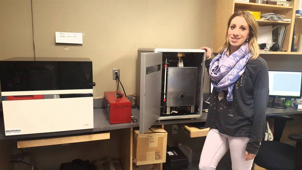
Figure 1: Elementar vario Pyro cube (right) coupled to an Isoprime VisION Mass Spectrometer (left)
Tree rings are a bio indicator of their surrounding environment and assist in climate reconstructions. They can provide an insight into seasonality, ecosystems and hydrological cycle functions in periods of climate change. We call the science of studying tree rings, dendrochronology. Although we can gain a ton of information from ring width variability alone, for example dry summers can lead to narrow ring widths and we summers to wide rings, we can also use stable isotopes of carbon δ 13C and oxygen δ 18O to investigate past precipitation and temperature regimes.
Methods
Methodological practices in stable isotope analysis involve sample collection, chemical pre-treatment, mass spectrometry and data analysis. Collection of tree ring samples depends on the type and the age of the wood. Modern samples are collected by coring trees using an increment borer to gather raw samples from desired trees and locations and then dating the years by crossdating (that is pattern matching the pattern of wide an narrow rings). Fossilized wood samples are collected as a whole disk, mostly because the trees are long dead and generally are dated using geochronology. Figure 2 illustrates modern tree core samples that have been mounted and sanded. Figure 3 illustrates fossilized wood samples. Samples are then mounted and sanded in preparation for milling.
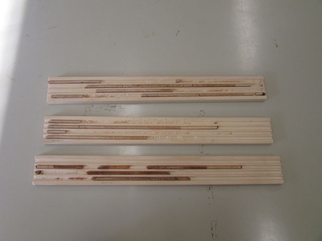
Figure 2: Modern Samples mounted and sanded
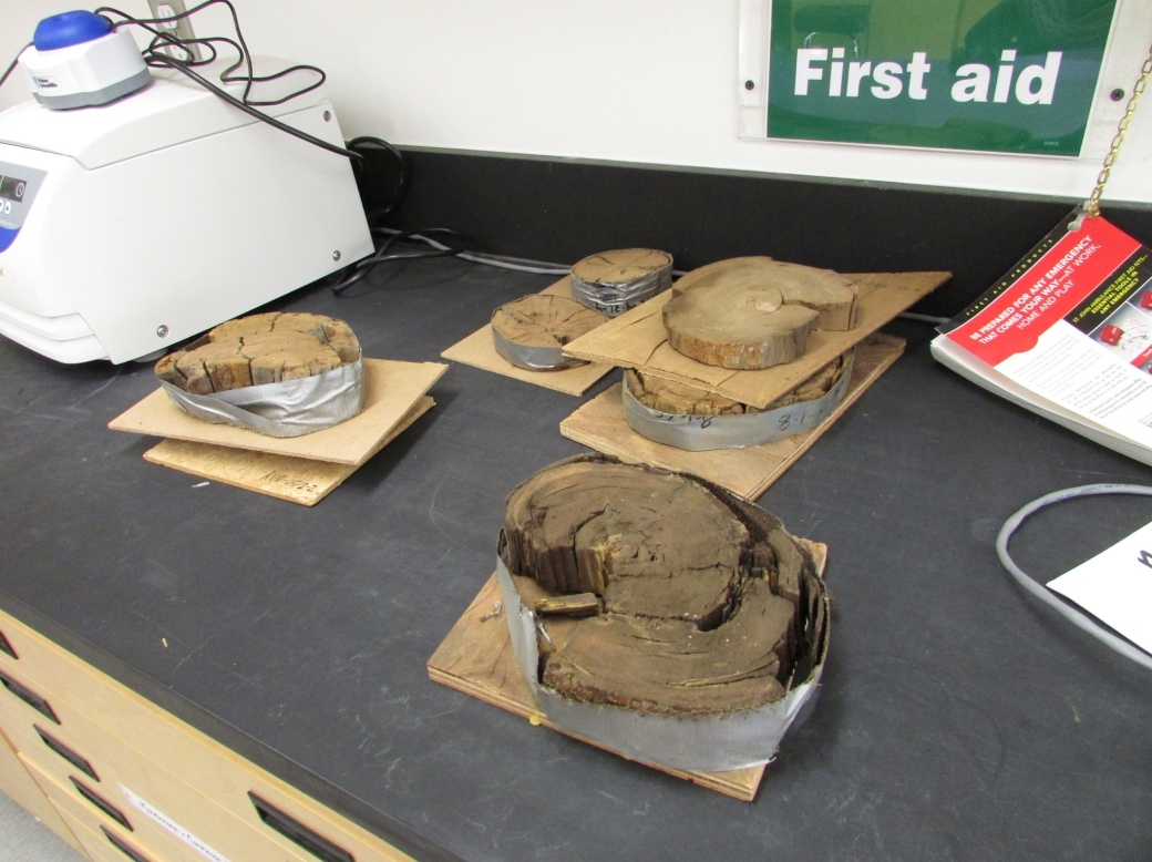
Figure 3: Fossilized wood samples
A micro miller is used to drill out each year (one tree ring), and with precision early wood and late wood can be collected. Figure 4 illustrates the micro miller used in the dendrochronology lab at Nipissing University.
Figure 4: Micro Miller
The shavings of raw wood from the micro miller are then gathered into vials. The raw wood samples are chemically processed to alpha cellulose. The samples are weighed into tin or silver capsules, depending on which isotope is being analyzed. Figured 5,6, and 7 visualize the final steps before the samples are entered into the Mass Spectrometer.
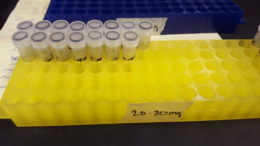
Figure 5: Raw wood shavings
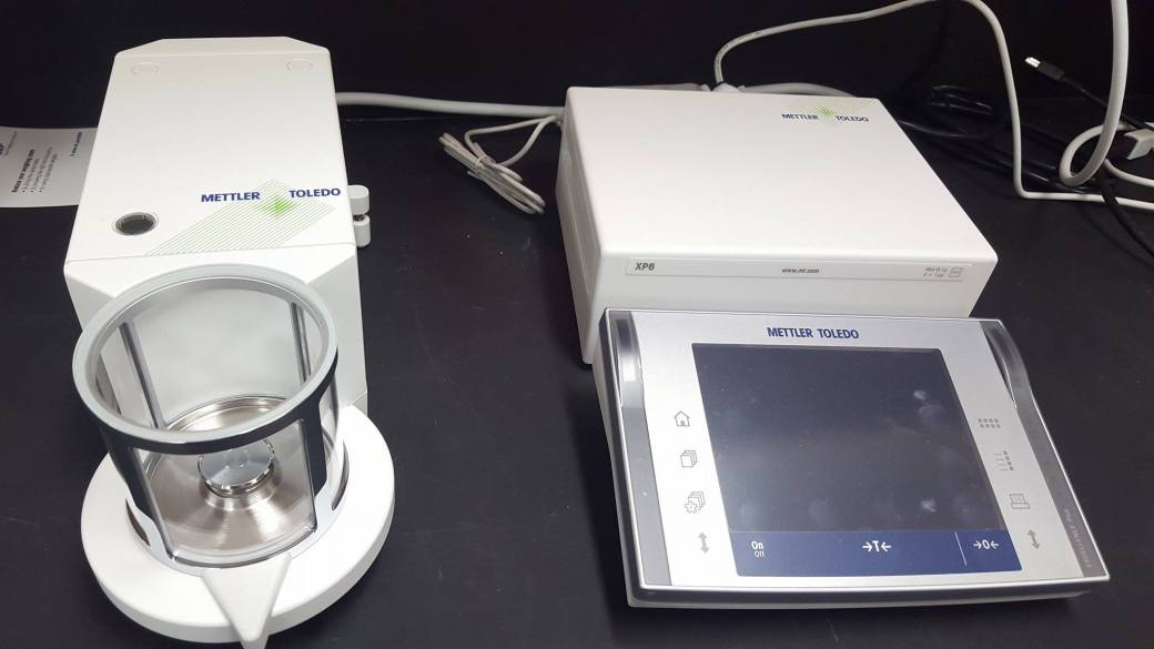
Figure 6: Micro scale
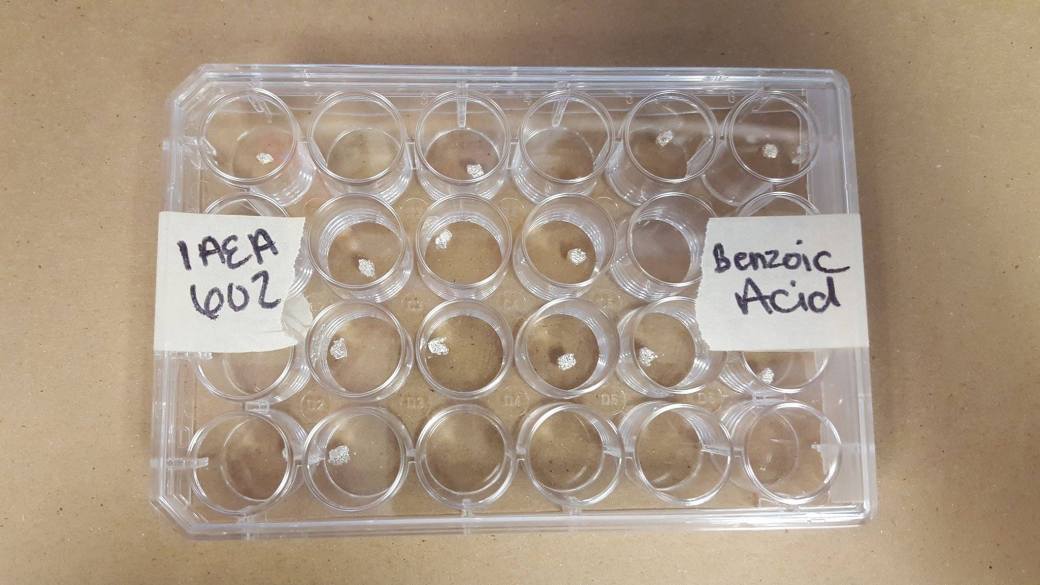
Figure 7: International standards in tin capsules ready to go into the Mass Spectrometer
How does a Mass Spectrometer work?
A Mass Spectrometer has the ability to analyze a variety of stable isotopes. The lab at Nipissing University primarily focuses on δ13C and δ180. The data that is generated is expressed as a ratio of parts per thousand ‰ (Figure 8). This is a value of the international standard which is a known isotopic value compared to the sample.

Figure 8: Final data generated from the Mass Spectrometer
(Good Practice Guide for Isotope Ratio Mass Spectrometry)
Samples are entered into the Elemental Analyzer auto sampler in either silver or tin capsules, depending on the isotopic analysis desired. In O and H mode (Oxygen and Hydrogen) samples are entered into the EA in silver capsules. A simplistic view of the sample analysis process is demonstrated in Figure 9.
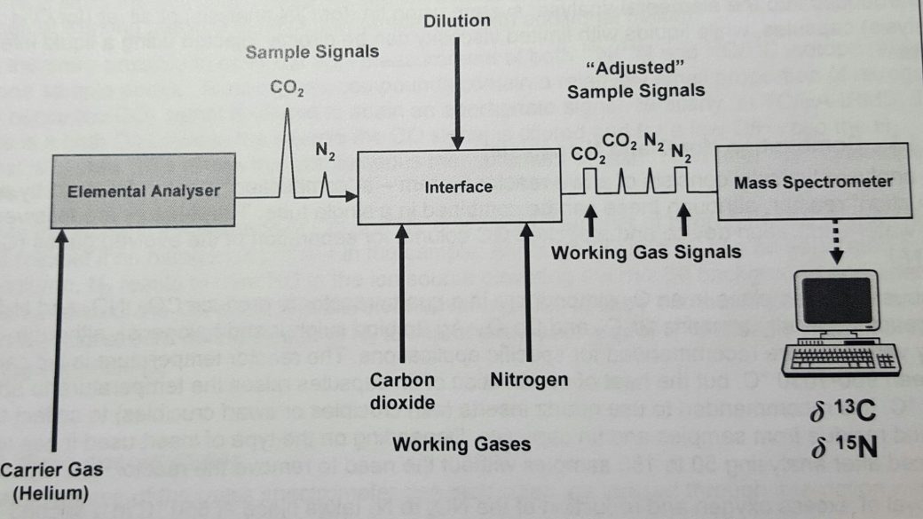
Figure 9: Mass Spectrometer analysis
(Good Practice Guide for Isotope Ratio Mass Spectrometry)
There are four primary steps to isotopic analysis. The first step involves combustion or thermal conversion of the sample material via the elemental analyzer. For example, H and O analysis mode high temperature conversion occurs around 13500C and 14500C. The column in the EA is packed with glassy carbon particles and silver wool to bind the hydrogen atoms. The evolved gasses are then separated via an isothermal packed column GC. Trapping materials such as Sicapent® are used to collect unwanted material (e.g. H2O) during analysis. Finally the gasses are released into the mass spectrometer by using a purge and trap method. This brings the samples to the second step, involving an introduction of the evolved gasses into the ion source of the mass spectrometer through the computer interface (Figure 10).
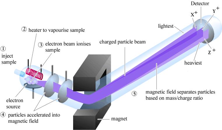
Figure 10: Reference Gasses (evolved gasses)
The third step positively ionizes the gas molecules and separates them by their masses, which is detected by faraday cups located in the Mass Spectrometer (Figure 11). The fourth step is the evaluation of raw data, which is generated as a ratio of parts per thousand.

Figure 11: Inside a Mass Spectrometer
(Good Practice Guide for Isotope Ratio Mass Spectrometry)
Dendro-provenancing using isotopes
Dendro-provenancing is a method where the pattern of tree ring widths can be used to identify where a specific wood sample has from. One of the limitations in this is that in order to figure this out you have to compare tree ring patterns against all the possible regions where the timber could have come from (Figure 11) . In many studies this is not difficult because timbers likely came from reasonably close to the location of the building but in Bermuda there are many possible sources of timber both in North America and Europe. To overcome this difficulty we plan to use isotopes. Because there are distinct regional patterns in stable isotopes, called isoscapes (Figure 12) we can use the isotopic value of the wood to narrow down the possible source region of the timber. Then we can enter the International Tree Ring Databank (ITRDB) and find chronologies from those regions against which we can match our timber ring width patterns and obtain a source region for the timber.
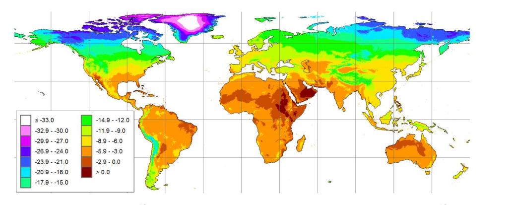
Figure 12: Isoscape map of δ180 (Terzer et al. (2013)
Reconstructing Plio-Pleistocene Climate in Alaska and the Yukon using δ 13C and δ 18O Isotopic Signatures of Larch (Larix lacricina)
The Arctic provides a stimulus to study climate change, as it is changing at a rapid rate. High latitude environments are an ideal geographic location to understand these chance as they reflect global evolution of Earth’s climate. To understand climatic and geochemical conditions of past environments, the analysis of the isotopic composition of ancient wood is a useful parameter. Highly resolved proxy records are a product of isotopic analysis and assist with climate reconstruction.
My thesis involves the analysis of stable isotopes δ13C and δ180 in order to reconstruct climate during the Plio-Pleistocene. The Plio-Pleistocene covers an important period of climatic change when there was a gradual cooling from a warmer period. Throughout the Arctic there exist numerous fossil forest sites from the Pliocene (2.6-5 million years ago) and Pleistocene (2.6 million – 10 thousand years ago) proving an opportunity to develop intra-annual records, through the use of tree-rings. Investigating climate change immediately prior to and during the onset of large scale northern hemisphere glaciation may give insight into climatic conditions being experience in the Artic today.
I will be using modern tree core samples and fossilized wood from Alaska and the Yukon to conduct my study. In this project, I expect to be able to produce seasonally resolved records of temperature and precipitation with the combination of isotopic data and tree ring widths.
Master’s of Environmental Science/Environmental Studies Graduate Program at Nipissing University
The MESc/MES graduate program at Nipissing University offers a unique program experienced catered to the individual interest of their students. I have had a variety of exceptional experiences. I feel I would not have been able to participate in these opportunities had I sought out a larger competitive institution.
In June 2015, I travelled to Reno, Nevada to understand chemical analysis of stable isotopes at the Desert Research Institution under the supervision of Dr. Adam Csank. During my time there I was able to experience the beautiful Lake Tahoe. I will be returning later this year to complete isotopic data analysis component of my research.
In August 2015, I had the opportunity to conduct a ten day climate-based research expedition in Denali National Park, Alaska with Dr. Stephanie McAfee and Dr. Adam Csank. It was an experience of a lifetime. Our Journey included Fairbanks and Anchorage. However the highlight of my trip was being able to take the 90mile road into the Natural Wildlife Preservation in Denali National Park. We stayed at Friday Creek Camp in Kantishna in the backcountry for four days at mile 90. We climbed three of the foothills while we there to set up climate recording instrumentation. However, the gem of this trip was being able to see Denali (the former Mount McKinley). After four days of constant rain (some hail) at camp, on the drive home she came out with all her glory! I hope to return later this year to collect additional samples, enhancing the overall outcome of my thesis.
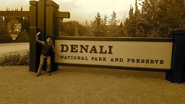
Figure 13: Entrance to Denali National Park, Alaska (Muldoon, 2015)
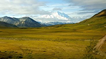
Figure 14: Denali, Denali National Park, Alaska (Muldoon, 2015)
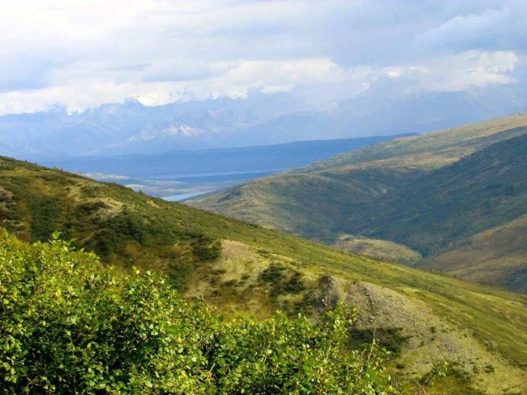
Figure 15: Katinshna Foothills Summit, Alaska (Muldoon, 2015)
Upcoming, I will have the opportunity to study at the University of Utah at the annual IsoCamp for two weeks in June 2016. I will have the opportunity to study amongst the top academics in the field of stable isotope analysis. I hope to be able to apply the knowledge gained at the camp to the dendroclimatology lab here at the university, at to branch out to other types of isotopic analysis in the isotope lab.
Furthermore, I have presented my thesis at the CAGONT conference in the fall of 2015 at Carleton University in Ottawa, Ontario. This spring I will present at the CAG (Canadian Association of Geographers) in Halifax, Nova Scotia.
I want to acknowledge and thank my supervisor Dr. Adam Csank for every one of these amazing opportunities during my time at Nipissing University and for his continuous support of my thesis. I would also like to thank Dr. April James for taking the co supervisory position and I look forward to her guidance through the final stages of this journey. I would also like to thank Dr. Stephanie McAfee for allowing me to assist on the Climate Research trip to Alaska.
